Matrix Factorization: QR Decomposition

Aside from LU decomposition we discussed previously, QR decomposition is another prominent method to decompose a matrix into a product of two matrices. In QR decomposition, a matrix \mathbf{A} is factorized into an orthogonal matrix \mathbf{Q} and an upper triangular matrix \mathbf{R} such that \mathbf{A} = \mathbf{Q}\mathbf{R}. QR decomposition can be applied to any square and rectangular matrix with linearly independent columns.

There are several ways of computing \mathbf{Q} and \mathbf{R}, namely the Gram–Schmidt process, Householder reflections, and Givens rotations. However, in this article, we focus on applying Householder reflections to compute such matrices, thanks to its simplicity and excellent numerical stability (the Gram–Schmidt process is known to be inherently unstable whereas the Givens rotations are significantly more complex to implement). For simplicity, let us assume that \mathbf{A} is square such that \mathbf{A}\in\mathbb{R}^{n\times n}. To find \mathbf{Q} and \mathbf{R}, we iteratively compute symmetric and orthogonal matrices \mathbf{Q}_i for i = 1,2,\hdots,n such that:

\underbrace{\mathbf{Q}_n\mathbf{Q}_{n-1}\cdots\mathbf{Q}_2\mathbf{Q}_1}_{\mathbf{Q}^\top}\mathbf{A} = \mathbf{R},

where \mathbf{Q}^\top = \mathbf{Q}_n\mathbf{Q}_{n-1}\cdots\mathbf{Q}_2\mathbf{Q}_1. The idea here is to transform each column of the original matrix such that the resulting column is zero below the main diagonal. To better illustrate how this works, suppose that we start with an unstructured matrix:

\mathbf{A} = \begin{bmatrix}* & * & * & \cdots & * \\ * & * & * & \cdots & * \\ * & * & * & \cdots & * \\ \vdots & \vdots & \vdots & \ddots & \vdots \\ * & * &* & \cdots & *\end{bmatrix},

where the symbol * represents any real number. Now we start with finding \mathbf{Q}_1 such that \mathbf{R}_1 is structured in the form of:

\mathbf{Q}_1\mathbf{A} = \underbrace{\begin{bmatrix}* & * & * & \cdots & * \\ 0 & * & * & \cdots & * \\ 0 & * & * & \cdots & * \\ \vdots & \vdots & \vdots & \ddots & \vdots \\ 0 & * &* & \cdots & *\end{bmatrix}}_{\mathbf{R}_1}.

Notice that the first column of the matrix \mathbf{R}_1 has zeros below the main diagonal. Next, we compute \mathbf{Q}_2 such that:

\mathbf{Q}_2\mathbf{Q}_1\mathbf{A} = \underbrace{\begin{bmatrix}* & * & * & \cdots & * \\ 0 & * & * & \cdots & * \\ 0 & 0 & * & \cdots & * \\ \vdots & \vdots & \vdots & \ddots & \vdots \\ 0 & 0 &* & \cdots & *\end{bmatrix}}_{\mathbf{R}_2}.

This process is repeated n times in total until we get \mathbf{R}_n that is an upper triangular matrix.

Now that we understand the big picture of the algorithm, the next important question is, how can we leverage the Householder reflection to find \mathbf{Q}_i? To be able to illustrate the mechanism of Householder reflection, let us restrict ourselves to the case where n = 2, i.e., two-dimensional case. The lecture by Toby Driscoll is an excellent source to understand the application of Householder reflection in QR decomposition. The main idea here is to treat the matrix \mathbf{Q}_i as a reflection operator to a particular mirror axis. In our case when \mathbf{A}\in\mathbb{R}^{2\times 2}, we want to find \mathbf{Q}_1 such that, when it is multiplied to the vector \mathbf{z} which represents the first column of \mathbf{A}, it gives:

\mathbf{Q}_1\mathbf{z} = \lVert \mathbf{z} \rVert_2\mathbf{e}_1,

where \mathbf{e}_i is the i-th standard basis vector. It is important to note that the above equation exists since \mathbf{Q}_1 must be orthogonal. From the above, we can clearly see that the operator \mathbf{Q}_1 somehow “moves” the vector \mathbf{z} into the axis in the first dimension. Define a new vector \mathbf{v} to represent the difference between the two, i.e.:

\mathbf{Q}_1\mathbf{z} = \lVert \mathbf{z} \rVert_2\mathbf{e}_1 = \mathbf{z} + \mathbf{v}.

The above vectors as well as the mirror are illustrated in the figure below:
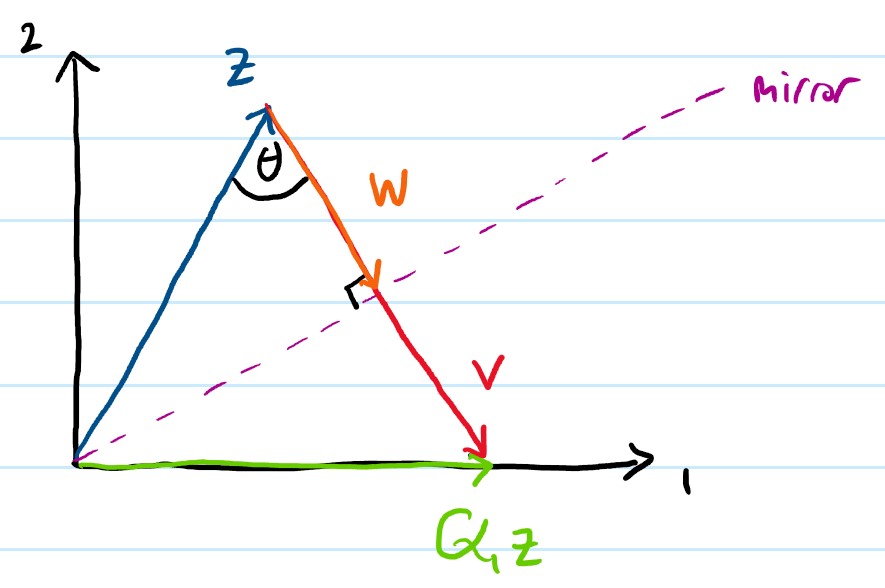
From the figure above, \mathbf{z} (blue) and \mathbf{Q}_1\mathbf{z} (green) are mirrors to each other with respect to the mirror axis (purple). We define an auxiliary vector \mathbf{w} (orange) which is simply a half of \mathbf{v} (red). Now, we want to find out what \mathbf{w} really is in terms of magnitude and angle. The magnitude (or the length) of \mathbf{w} is equal to:

\lVert \mathbf{w} \rVert_2 = \lVert \mathbf{z} \rVert_2 cos(\theta) = \lVert \mathbf{z} \rVert_2 \left(-\frac{\mathbf{z}^\top\mathbf{v}}{\lVert \mathbf{z} \rVert_2 \lVert \mathbf{v} \rVert_2 } \right) = -\frac{\mathbf{z}^\top\mathbf{v}}{ \lVert \mathbf{v} \rVert_2 } .

Instead of finding the angle (or direction) of \mathbf{w}, we can simply use the unit vector of \mathbf{v}. As such, \mathbf{w} is simply:

\mathbf{w} = \lVert \mathbf{w} \rVert_2 \frac{\mathbf{v}}{ \lVert \mathbf{v} \rVert_2 } = -\frac{\mathbf{z}^\top\mathbf{v}}{ \lVert \mathbf{v} \rVert_2 }\frac{\mathbf{v}}{ \lVert \mathbf{v} \rVert_2 } = -\mathbf{v}\frac{\mathbf{z}^\top\mathbf{v}}{ \lVert \mathbf{v} \rVert_2^2 }.

This results in:

\mathbf{Q}_1\mathbf{z} = \mathbf{z} + \mathbf{v} = \mathbf{z} + 2\mathbf{w} = \mathbf{z} -2\mathbf{v}\frac{\mathbf{z}^\top\mathbf{v}}{ \lVert \mathbf{v} \rVert_2^2 } = \left(\mathbf{I}-2\frac{\mathbf{v}\mathbf{v}^\top}{\mathbf{v}^\top\mathbf{v}}\right)\mathbf{z},

which implies that:

\mathbf{Q}_1 = \mathbf{I}-2\frac{\mathbf{v}\mathbf{v}^\top}{\mathbf{v}^\top\mathbf{v}},

where \mathbf{v} = \lVert \mathbf{z} \rVert_2\mathbf{e}_1-\mathbf{z}. One can easily confirm by the definition of orthogonality that \mathbf{Q}_1 is in fact orthogonal.

The above process is repeated to obtain \mathbf{Q}_2 and so on until \mathbf{Q}_n. However, since we do not want to change the previously computed columns, one only needs to apply the Householder reflection to the remaining rows (from the main diagonal to the end). I would recommend you to also check out the Wikipedia page about QR decomposition for some numerical examples.

Matrix Factorization: LU Decomposition

LU (short for lower-upper) decomposition is a form of matrix factorization that decomposes a matrix into a product of lower and upper triangular matrices. This matrix factorization approach was introduced by the Polish astronomer Tadeusz Banachiewicz in 1938. In a way, LU decomposition can be seen as a Gaussian elimination (row reduction) method executed in matrix form. The LU decomposition is one of the most widely used matrix factorization methods for solving a system of linear equations (realize that such problems arise in many different fields including engineering, physics, economics, computer science, and applied mathematics), especially when such a system results in an equation \mathbf{A}\mathbf{x}=\mathbf{b} where \mathbf{A}\in\mathbb{R}^{n\times n} is square and known, \mathbf{b}\in\mathbb{R}^n is given, and \mathbf{x}\in\mathbb{R}^n is the variable to be solved.

In this article, we will discuss the steps to execute an LU decomposition algorithm on a square matrix \mathbf{A} such that it can be written as \mathbf{A} = \mathbf{L} \mathbf{U} for a lower triangular matrix \mathbf{L}\in\mathbb{R}^{n\times n} and an upper triangular matrix \mathbf{U}\in\mathbb{R}^{n\times n}. However, note that, when \mathbf{A} has at least a zero on the main diagonal, then one needs to interchange either some of its row or column, and this will involve a row permutation matrix \mathbf{P}\in\mathbb{R}^{n\times n} or a column permutation matrix \mathbf{Q}\in\mathbb{R}^{n\times n} that are not equal to the identity matrix. However, for the sake of simplicity, let us assume for now that the main diagonal of \mathbf{A} has no zero entries.

The Wikipedia page on LU decomposition is an excellent starting point for understanding the mechanics of this factorization method. Following some of the notations, let us assume that we have a square matrix \mathbf{A}\in\mathbb{R}^{n\times n} having no zero on the diagonal. As such, denote \mathbf{A}^{(i)} as the i-th version of \mathbf{A} where all of the elements below its main diagonal have been eliminated to zero through the row reduction method for the first i-th columns. Then, at step i, we have \mathbf{A}^{(i)} =  \mathbf{L}_{i}^{-1}\mathbf{A}^{(i-1)} where \mathbf{L}_{i}^{-1} is an identity matrix with the exception that its entries below the diagonal at the i-$th column are (most likely) nonzero. Starting from \mathbf{A}^{(0)} = \mathbf{A}, then we carried out the following steps until n-1:

\mathbf{A} =  \mathbf{L}_{1}\mathbf{L}_{1}^{-1}\mathbf{A}^{(0)}=\mathbf{L}_{1}\mathbf{A}^{(1)} \Leftrightarrow \mathbf{A} =  \mathbf{L}_{1}\mathbf{L}_{2}\mathbf{L}_{2}^{-1}\mathbf{A}^{(1)}=\mathbf{L}_{1}\mathbf{L}_{2}\mathbf{A}^{(2)} \Leftrightarrow \cdots \Leftrightarrow \mathbf{A}  =\mathbf{L}_{1}\mathbf{L}_{2}\hdots\mathbf{L}_{n-1}\mathbf{A}^{(n-1)},

which suggest that \mathbf{L} \triangleq \mathbf{L}_{1}\mathbf{L}_{2}\hdots\mathbf{L}_{n-1} and \mathbf{U} \triangleq\mathbf{A}^{(n-1)}.

To illustrate how the above makes sense in the LU decomposition algorithm, let us consider a simple example where \mathbf{A}\in\mathbb{R}^{3\times 3} is given as:

\mathbf{A}= \begin{bmatrix}1 & -1 & 0\\0 & 3 & 1\\0.5&2&2\end{bmatrix}.

Firstly, we do the row reduction on the first column. This is performed as follows:

\begin{bmatrix}1 & -1 & 0\\0 & 3 & 1\\0&2.5&2\end{bmatrix} = \begin{bmatrix}1 & -1 & 0\\0 & 3 & 1\\0.5&2&2\end{bmatrix} - \begin{bmatrix}0& 0 & 0\\\frac{0}{1}(1) & \frac{0}{1}(-1)& \frac{0}{1}(0)\\\frac{1}{2}(1) & \frac{1}{2}(-1)& \frac{1}{2}(0)\end{bmatrix},

which is equal to:

\underbrace{\begin{bmatrix}1 & -1 & 0\\0 & 3 & 1\\0&2.5&2\end{bmatrix}}_{\mathbf{A}^{(1)}}= \underbrace{\begin{bmatrix}1 & 0 & 0\\0 & 1 & 0\\-0.5&0&1\end{bmatrix}}_{\mathbf{L}^{-1}_1}\underbrace{\begin{bmatrix}1 & -1 & 0\\0 & 3 & 1\\0.5&2&2\end{bmatrix}}_{\mathbf{A}^{(0)}}.

Thanks to the lower triangular structure of \mathbf{L}^{-1}_1, then it is easy to verify that its inverse, \mathbf{L}_1, is equal to:

\mathbf{L}_1=\begin{bmatrix}1 & 0 & 0\\0 & 1 & 0\\0.5&0&1\end{bmatrix}.

Secondly, we repeat the same step but on the second column. This results in:

\begin{bmatrix}1 & -1 & 0\\0 & 3 & 1\\0&0&1.1667\end{bmatrix} = \begin{bmatrix}1 & -1 & 0\\0 & 3 & 1\\0&2.5&2\end{bmatrix} - \begin{bmatrix}0& 0 & 0\\0 & 0& 0\\\frac{5}{6}(0) & \frac{5}{6}(3)& \frac{5}{6}(1)\end{bmatrix},

which is equal to:

\underbrace{\begin{bmatrix}1 & -1 & 0\\0 & 3 & 1\\0&0&1.1667\end{bmatrix}}_{\mathbf{A}^{(2)}}= \underbrace{\begin{bmatrix}1 & 0 & 0\\0 & 1 & 0\\0&-\frac{5}{6}&1\end{bmatrix}}_{\mathbf{L}^{-1}_2}\underbrace{\begin{bmatrix}1 & -1 & 0\\0 & 3 & 1\\0&2.5&2\end{bmatrix}}_{\mathbf{A}^{(1)}}.

Again, it is straightforward to verify that \mathbf{L}_2 is simply equal to:

\mathbf{L}_2=\begin{bmatrix}1 & 0 & 0\\0 & 1 & 0\\0&\frac{5}{6}&1\end{bmatrix}.

That’s it! Now we are ready to compute the LU decomposition. The matrix \mathbf{L} is equal to:

\mathbf{L}=  \mathbf{L}_1\mathbf{L}_2= \begin{bmatrix}1 & 0 & 0\\0 & 1 & 0\\0.5&\frac{5}{6}&1\end{bmatrix}= \begin{bmatrix}1 & 0 & 0\\0 & 1 & 0\\0.5&0.8333&1\end{bmatrix},

whereas \mathbf{U} is nothing but:

\mathbf{U}=  \mathbf{A}^{(2)}= \begin{bmatrix}1 & -1 & 0\\0 & 3 & 1\\0&0&1.1667\end{bmatrix}.

At last, we finally have:

\underbrace{\begin{bmatrix}1 & -1 & 0\\0 & 3 & 1\\0.5&2&2\end{bmatrix}}_{\mathbf{A}}= \underbrace{\begin{bmatrix}1 & 0 & 0\\0 & 1 & 0\\0.5&0.8333&1\end{bmatrix}}_{\mathbf{L}}\underbrace{\begin{bmatrix}1 & -1 & 0\\0 & 3 & 1\\0&0&1.1667\end{bmatrix}}_{\mathbf{U}}.

Pretty easy, right? Now I want to mention that the process above, which is called the pure LU decomposition, will only work when there is no zero on the main diagonal, or in more technical terms, all its leading principal minors are nonzero. A generalization of LU decomposition is the LUP decomposition, where the letter P here denotes the row permutation matrix. LUP is simply an LU decomposition but with partial pivoting (row). That is, LU decomposition is equal to LUP decomposition in which the permutation matrix is equal to the identity matrix. The aforementioned Wikipedia page on the LU decomposition neatly covers an example of how the LUP decomposition is performed.

Hopefully, this short article can help you in understanding the LU decomposition. For the next articles, I am planning on explaining how the QR decomposition works and comparing the performance between LU and QR decomposition to solve some systems of linear equations on an embedded system. Stay tuned!